The Huber loss
You will learn
How the Huber loss treats a small error like squared error and a large one linearly, so outliers pull less.
Squared error lets one outlier dominate: an error of 3 costs 4.5 as half its square, as much as 36 errors of 0.5. Huber is half the square while |e| is within delta and then grows only linearly, delta |e| - delta^2 / 2, so with delta 1 that error costs 2.5. The two pieces meet with the same value and slope, and the gradient never grows past delta: a far-off point pulls on the model with a bounded force. For the spec's pair of errors 0.5 and 3 the mean is 1.3125, against 2.3125 for half the square. The spec huber_loss.t27 computes both.
Try it
Set delta to 0.5 and drag the error to 3; then find where the two curves part.
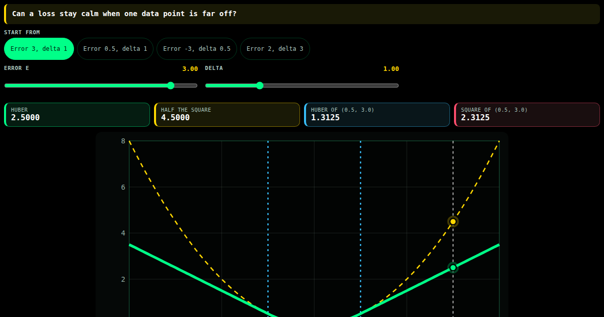
Drag the error along: Huber is half its square inside delta and only grows linearly outside, so one wild miss pulls on the model with a bounded force. The dashed curve is the pure square.
specs/ml/loss/huber_loss.t27
// SPDX-License-Identifier: Apache-2.0
// t27/specs/
// Threshold where loss changes from quadratic to linear | φ² + 1/φ² = 3 | TRINITY
// Restored 2026-10-05 from trinity specs/algo/huber_loss.tri: the port kept only
// the first parameter and returned void, so forward computed a value and
// threw it away, and every test asserted `result != undefined`.

module HuberLoss;
    use base::types;
    use math::constants;

    // ═══════════════════════════════════════════════════════════
    // 2. Types
    // ═══════════════════════════════════════════════════════════

    pub const HuberLossConfig = struct {
        delta : f32,
    };

    // ═══════════════════════════════════════════════════════════
    // 3. Core Functions
    // ═══════════════════════════════════════════════════════════

    // per element e = prediction - target:
    //   |e| <= delta: 0.5 e^2      else: delta |e| - 0.5 delta^2
    fn element_loss(e: f32, delta: f32) -> f32 {
        const a = @abs(e);
        if (a <= delta) {
            return 0.5 * e * e;
        }
        return delta * a - 0.5 * delta * delta;
    }

    // forward(predictions, targets, delta) -> f32. The .tri gives the
    // per-element formula only; this returns the MEAN over elements
    // (PyTorch HuberLoss default reduction). 0 for n = 0.
    fn forward(predictions: []const f32, targets: []const f32, delta: f32) -> f32 {
        if (predictions.len == 0) {
            return 0.0;
        }
        var sum_loss : f32 = 0.0;
        var i : usize = 0;
        while (i < predictions.len) {
            sum_loss = sum_loss + element_loss(predictions[i] - targets[i], delta);
            i = i + 1;
        }
        return sum_loss / (predictions.len as f32);
    }

    // ═══════════════════════════════════════════════════════════
    // TDD: Tests
    // ═══════════════════════════════════════════════════════════

    fn huber_one(e: f32, delta: f32) -> f32 {
        const predictions : [1]f32 = [e];
        const targets : [1]f32 = [0.0];
        return forward(&predictions, &targets, delta);
    }

    test quadratic_inside_delta
        given result = huber_one(0.5, 1.0)
        when negative = huber_one(-0.5, 1.0)
        then @abs(result - 0.125) < 0.000001 and result == negative

    // delta |e| - delta^2 / 2 = 3 - 0.5
    test linear_outside_delta
        given result = huber_one(3.0, 1.0)
        when wide = huber_one(3.0, 2.0)
        then @abs(result - 2.5) < 0.000001 and @abs(wide - 4.0) < 0.000001

    // the two pieces meet with equal value and slope at |e| = delta
    test continuous_at_delta
        given below = huber_one(0.999, 1.0)
        when above = huber_one(1.001, 1.0)
        then @abs(above - below - 0.002) < 0.0001

    // mean of (0.125, 2.5) over two elements
    fn huber_two(e0: f32, e1: f32, delta: f32) -> f32 {
        const predictions : [2]f32 = [e0 + 1.0, e1 + 1.0];
        const targets : [2]f32 = [1.0, 1.0];
        return forward(&predictions, &targets, delta);
    }

    test forward_mean
        given result = huber_two(0.5, 3.0, 1.0)
        when expected = 1.3125
        then @abs(result - expected) < 0.000001

    // ═══════════════════════════════════════════════════════════
    // TDD: Invariants
    // ═══════════════════════════════════════════════════════════

    invariant huber_zero_at_target
        assert huber_one(0.0, 1.0) == 0.0
All lessons
Module 1 · One neuron
A neuron sums its inputs and bends the sum: ReLU, the sigmoid and tanh, and where each one stops passing a gradient back.
Module 2 · New bends
The smooth curves of current models: GELU with its dip, Swish with its knob, and ELU with a floor instead of a cliff.
Module 3 · A layer
What sits around the neurons: softmax turns scores into a choice, an embedding turns a word into numbers, dropout switches units off.
Module 4 · Pictures
Reading a picture in patches: a window averaged over its patch, max pooling, and batch normalisation of features on different scales.
Module 5 · The error
How wrong a guess is, as one number: mean squared error, cross-entropy for probabilities, and the Huber loss for outliers.
Module 6 · Downhill
Walking down the loss: gradient descent with momentum, RMSProp that ignores the gradient's size, and Adam that combines them.
Module 7 · Learning
Where the gradients come from and what they achieve: backpropagation through a layer, a network that learns XOR, and LAMB for large batches.
Module 8 · Memory and attention
Networks that read a sequence: a recurrent cell and its fading echo, the gates of an LSTM, and attention over every position at once.
Module 9 · The transformer and the reward
The parts of a transformer and of an agent: positions as clocks, one encoder block, and PPO, which learns from reward without lurching.